Prerequisites: Joins and Big O
Why a join loses rows, why it multiplies them, and why an index decides if it finishes
What this lesson covers
- A join multiplies rows, and that is how totals go wrong
- The filter that silently turns LEFT JOIN into INNER JOIN
- Finding what is missing, not what matches
- A spatial join is a join with a predicate in ON
- Why the index is the difference between 72 ms and a timeout
Run the query below.
It returns a hundred named things — cafés, benches, post boxes, shrines — from six square kilometres of central Tokyo, and the map draws them where they stand. There are 2,184 of them in that box, of 75 different kinds.
That cost nothing to set up. No Docker, no download, no ogr2ogr, no waiting: the OpenStreetMap extract behind it holds 440 million buildings and it is already connected. Every query on this page runs against it, and every one of them is yours to edit.
Then come the questions that first result raises — and they are the rest of this lesson:
- What if I want the parcels, and what is inside each one?
- Why did moving one condition from
ONtoWHEREdelete thirty of my rows? - Why is one parcel’s area coming back sixty-six times too large?
- Why does the same query hang for thirty seconds if I drop the bounding box?
Two ideas answer all four, and neither is about geography: a join decides which rows survive — and quietly multiplies them — and an index decides whether that join finishes at all. A spatial join is an ordinary join whose ON clause reads ST_Contains(…) instead of a.id = b.id, so every rule and every trap carries straight over.
A hundred named things in central Tokyo
SELECT name, osm_type, geom
FROM osm.amenity_point
WHERE geom && ST_MakeEnvelope(139.75, 35.67, 139.78, 35.69, 4326)
  AND name IS NOT NULL
LIMIT 100;
Five lines, one table, no joins and no functions except the one that draws the box. && compares bounding boxes against the index, which is why this returns in milliseconds against a 440-million-row database. It selects geom, so the result is geometry — not a table about places, the places themselves.
Not required reading
These lessons are for running queries, reading rows and pushing them onto the map as a layer — not for studying theory first. Skip ahead and come back when a query returns a number you do not believe, or sits there for thirty seconds.
Now the parcels, and what is inside each one
WITH box AS (
    SELECT ST_MakeEnvelope(139.75, 35.67, 139.78, 35.69, 4326) AS g
),
parcels AS (
    SELECT l.osm_id, l.name, l.geom
    FROM osm.landuse_polygon AS l, box
    WHERE l.geom && box.g AND l.name IS NOT NULL AND l.name <> ''
)
SELECT p.name                              AS parcel,
       count(a.osm_id)                     AS amenities,
       round(ST_Area(p.geom::geography))   AS area_m2,
       p.geom
FROM parcels AS p
LEFT JOIN osm.amenity_point AS a ON ST_Contains(p.geom, a.geom)
GROUP BY p.osm_id, p.name, p.geom
ORDER BY amenities DESC
LIMIT 50;
The first question from the intro. This is a spatial join: osm.landuse_polygon on the left, osm.amenity_point on the right, matched by ST_Contains instead of by an id. It is a LEFT JOIN, so a parcel holding nothing still appears — with a count of 0 rather than vanishing. It returns geom too, so this one is also a layer.
Joins, in one page
A spatial join is an ordinary join. The only difference is the matching condition:
ON o.customer_id = c.id                        -- ordinary
ON ST_Contains(parcel.geom, amenity.geom)      -- spatial
Everything below is true of both. The two mistakes at the end are not join trivia — they are the two ways a spatial query returns a confident, wrong answer.
Which rows survive
| Join | Keeps | Unmatched rows |
|---|---|---|
INNER JOIN |
rows matching on both sides | dropped |
LEFT JOIN |
every row on the left | right columns become NULL |
FULL OUTER JOIN |
every row from either side | missing side becomes NULL |
CROSS JOIN |
every combination | nothing matches, so nothing drops |
RIGHT JOIN is LEFT JOIN with the tables swapped. Full reference: PostgreSQL — joined tables.
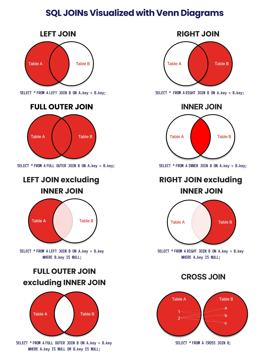
The abstract shape, with three customers and three orders — one customer has two orders, and one order belongs to a customer who does not exist:
-- INNER: only Alice, twice. Bob, Cara and the orphan order all disappear.
SELECT c.name, o.id
FROM customers AS c
JOIN orders AS o ON o.customer_id = c.id;

-- LEFT: all three customers; Bob and Cara get NULL order columns.
SELECT c.name, o.id
FROM customers AS c
LEFT JOIN orders AS o ON o.customer_id = c.id;
Those two tables do not exist in this database — they are the picture. Every query you can run on this page uses the real thing: osm.landuse_polygon as the parcels and osm.amenity_point as what is inside them, both filtered to one bounding box in central Tokyo. In that box there are 342 landuse polygons, of which 34 carry a name.
Mistake 1 — the filter in the wrong clause
LEFT JOIN promises to keep every left row. A condition on the right table in WHERE breaks that promise, because NULL fails every comparison:
-- keeps all 34 parcels; those with no café simply have NULL on the right
LEFT JOIN osm.amenity_point AS a
  ON ST_Contains(p.geom, a.geom)
 AND a.osm_type = 'cafe'

-- silently an INNER JOIN: only the 4 parcels that do have a café survive
LEFT JOIN osm.amenity_point AS a ON ST_Contains(p.geom, a.geom)
WHERE a.osm_type = 'cafe'
Nothing errors. The row count drops from 34 to 4, and "parcels and their cafés" quietly becomes "parcels that have a café".
Filter the right table in ON. Filter the left table in WHERE.
Mistake 2 — rows multiply
A parcel containing 66 amenities produces 66 rows. Anything you sum over those rows is counted 66 times — including the parcel's own area, which has not changed at all:
SELECT p.name,
       count(*)              AS rows_the_join_made,
       round(p.area_m2)      AS area_m2_once,
       round(sum(p.area_m2)) AS area_m2_if_you_sum_it   -- 66× too big
FROM parcels AS p
JOIN osm.amenity_point AS a ON ST_Contains(p.geom, a.geom)
GROUP BY p.osm_id, p.name, p.area_m2;
count(*) counts join rows. count(a.osm_id) counts matches and ignores the NULL a LEFT JOIN inserts — so an empty parcel scores 0 rather than 1. When you only need to know whether something is inside, EXISTS never multiplies anything.
Finding what is missing
Which parcels contain nothing at all? An inner join cannot answer this — the rows it would need are exactly the ones it drops:
SELECT p.name, p.geom
FROM parcels AS p
WHERE NOT EXISTS (
    SELECT 1 FROM osm.amenity_point AS a WHERE ST_Contains(p.geom, a.geom)
);
19 of the 34. That is the bottom half of the diagram — the shapes with the overlap removed — and because it returns geom, it is a layer you can put on the map.
In SedonaDB the join types and both mistakes are identical; it is the same SQL dialect over files instead of tables. What differs is which predicates it can accelerate: Sedona — spatial join optimizer.
INNER JOIN — and the 30 parcels it deletes
WITH box AS (
    SELECT ST_MakeEnvelope(139.75, 35.67, 139.78, 35.69, 4326) AS g
),
parcels AS (
    SELECT l.osm_id, l.name, l.geom
    FROM osm.landuse_polygon AS l, box
    WHERE l.geom && box.g AND l.name IS NOT NULL AND l.name <> ''
)
SELECT p.name              AS parcel,
       a.name              AS cafe,
       a.osm_subtype       AS kind
FROM parcels AS p
JOIN osm.amenity_point AS a
  ON ST_Contains(p.geom, a.geom)
 AND a.osm_type = 'cafe'
ORDER BY p.name, a.name
LIMIT 50;
The same two tables, joined the ordinary way and filtered to cafés. An inner join keeps only pairs that match on both sides, so a parcel with no café is not "a parcel with zero cafés" — it is gone. Four of the thirty-four parcels survive; the other thirty are simply absent from the result, with nothing to indicate they ever existed.
The 19 parcels with nothing inside
WITH box AS (
    SELECT ST_MakeEnvelope(139.75, 35.67, 139.78, 35.69, 4326) AS g
),
parcels AS (
    SELECT l.osm_id, l.name, l.geom
    FROM osm.landuse_polygon AS l, box
    WHERE l.geom && box.g AND l.name IS NOT NULL AND l.name <> ''
)
SELECT p.name                            AS parcel,
       round(ST_Area(p.geom::geography)) AS area_m2,
       p.geom
FROM parcels AS p
WHERE NOT EXISTS (
    SELECT 1
    FROM osm.amenity_point AS a
    WHERE ST_Contains(p.geom, a.geom)
)
ORDER BY area_m2 DESC
LIMIT 50;
The question an inner join structurally cannot answer, because the rows it needs are the ones it drops. NOT EXISTS asks it directly and stops at the first match, so it never builds the join and never multiplies anything. This is the bottom half of the Venn diagram — the shapes with the overlap removed — and it is often the more interesting half.
The trap: the same filter, in ON and in WHERE
WITH box AS (
    SELECT ST_MakeEnvelope(139.75, 35.67, 139.78, 35.69, 4326) AS g
),
parcels AS (
    SELECT l.osm_id, l.name, l.geom
    FROM osm.landuse_polygon AS l, box
    WHERE l.geom && box.g AND l.name IS NOT NULL AND l.name <> ''
),
filter_in_on AS (
    SELECT p.osm_id
    FROM parcels AS p
    LEFT JOIN osm.amenity_point AS a
      ON ST_Contains(p.geom, a.geom)
     AND a.osm_type = 'cafe'
    GROUP BY p.osm_id
),
filter_in_where AS (
    SELECT p.osm_id
    FROM parcels AS p
    LEFT JOIN osm.amenity_point AS a
      ON ST_Contains(p.geom, a.geom)
    WHERE a.osm_type = 'cafe'
    GROUP BY p.osm_id
)
SELECT 'osm_type = cafe in ON'    AS filter_placement,
       count(*)                   AS parcels_returned
FROM filter_in_on
UNION ALL
SELECT 'osm_type = cafe in WHERE',
       count(*)
FROM filter_in_where;
Both halves of this query are a LEFT JOIN with osm_type = 'cafe'. The only difference is which clause the condition sits in. In ON it is part of the match, so unmatched parcels survive with NULL on the right. In WHERE it runs after the join, and NULL fails every comparison — so the rows the LEFT JOIN just created are deleted again and you have an inner join wearing a LEFT JOIN's clothes.
A join multiplies rows — and your totals with them
WITH box AS (
    SELECT ST_MakeEnvelope(139.75, 35.67, 139.78, 35.69, 4326) AS g
),
parcels AS (
    SELECT l.osm_id, l.name, l.geom,
           ST_Area(l.geom::geography) AS area_m2
    FROM osm.landuse_polygon AS l, box
    WHERE l.geom && box.g AND l.name IS NOT NULL AND l.name <> ''
)
SELECT p.name                      AS parcel,
       count(*)                    AS rows_the_join_made,
       round(p.area_m2)            AS area_m2_once,
       round(sum(p.area_m2))       AS area_m2_if_you_sum_it
FROM parcels AS p
JOIN osm.amenity_point AS a ON ST_Contains(p.geom, a.geom)
GROUP BY p.osm_id, p.name, p.area_m2
ORDER BY rows_the_join_made DESC
LIMIT 10;
Chiyoda contains 66 amenities, so the join emits 66 rows for it, each carrying a full copy of the parcel — including its area. Sum that column and you have added the same 1.4 km² sixty-six times. Nothing about the query looks wrong, and the result is off by a factor of 66. This is the single most common way a correct-looking spatial join produces a wrong number.
Now make the ON clause spatial
Everything above holds with one substitution:
ON o.customer_id = c.idbecomesON ST_Contains(parcel.geom, amenity.geom). Same join types, same NULL rules, same row multiplication.What changes is the price of one comparison — and that is the second idea.
Four desktop steps as one statement
WITH box AS (
    SELECT ST_MakeEnvelope(139.75, 35.67, 139.78, 35.69, 4326) AS g
),
parcels AS (
    SELECT l.osm_id, l.name, l.geom
    FROM osm.landuse_polygon AS l, box
    WHERE l.geom && box.g AND l.name IS NOT NULL AND l.name <> ''
)
SELECT p.name        AS parcel,
       a.osm_type    AS category,
       count(*)      AS amenities
FROM parcels AS p
JOIN osm.amenity_point AS a ON ST_Contains(p.geom, a.geom)
GROUP BY p.osm_id, p.name, a.osm_type
ORDER BY amenities DESC
LIMIT 30;
Select by location, join, group, order — a four-step point-and-click workflow written once. The extra dimension here is osm_type, so each row is a parcel-and-category pair rather than a parcel total. This is the argument for spatial SQL over a desktop GIS: a query is versionable, diffable and re-runnable tomorrow, and a click history is none of those.
Why some queries never finish
You need none of this to write spatial SQL. You need it the first time a query hangs for thirty seconds and you have to guess why.
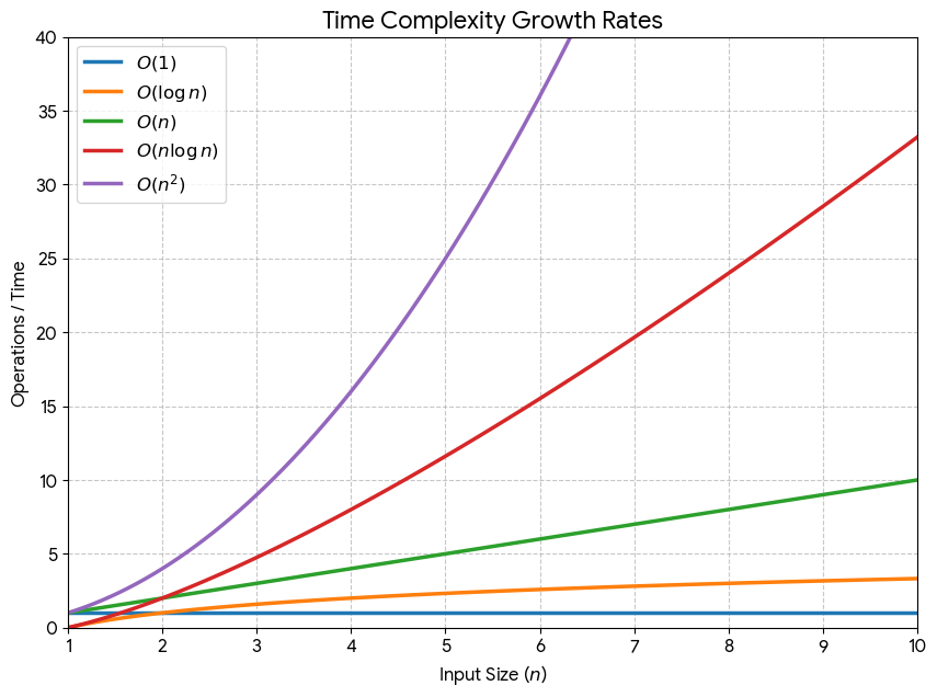
The curve a query lands on is decided by one thing: whether an index can answer its ON clause.
| Growth | What it means | Where you meet it |
|---|---|---|
O(log n) |
each step halves the candidates | an index probe |
O(n) |
every row, once | a sequential scan |
O(n × m) |
every left row against every right row | a join with no usable index |
The first two are fine at any size here. The third is the cliff.
The number that decides everything
osm.building_polygon 440,727,425 rows
Join that to anything without an index and you are asking for hundreds of billions of comparisons. The editor cancels the statement at 30 seconds, so what you actually see is a query that "doesn't work".
This is why every query in these lessons carries a bounding box:
WHERE geom && ST_MakeEnvelope(139.75, 35.67, 139.78, 35.69, 4326)
Same query, 72 ms instead of never.
What the index actually does
A GIST index stores each geometry's bounding box in a tree, so instead of scanning m rows the database descends it. On the small box used in this lesson — 342 polygons, 2,184 points:
no index    342 × 2,184        = 746,928 comparisons
index       342 × log₂(2,184)  ≈   3,794 comparisons   (~197× less)
And the gap widens as the data grows, because one side is a logarithm. See PostgreSQL — index types and PostGIS — spatial indexing.
Why && comes first
PostGIS splits every spatial predicate in two:
&&compares bounding boxes — cheap, and the index can answer it.ST_Containscompares real geometry — exact, and a 500-vertex polygon costs 500 vertices of arithmetic.
The planner runs the cheap one first and the exact one only on the survivors. Defeat the index — wrap the geometry column in a function, compare across mismatched SRIDs — and you drop back onto the steep curve, with nothing to warn you except the wait.
To see which path a query actually took, ask: PostgreSQL — using EXPLAIN.
In SedonaDB there is no GIST index; it partitions and builds an index per query instead, and only for predicates it recognises — Sedona — spatial join optimizer. The lesson is the same: a join it cannot accelerate is a join that compares every pair.
Why && runs before ST_Contains
WITH box AS (
    SELECT ST_MakeEnvelope(139.75, 35.67, 139.78, 35.69, 4326) AS g
),
land AS (
    SELECT l.osm_id, l.geom
    FROM osm.landuse_polygon AS l, box
    WHERE l.geom && box.g AND l.name IS NOT NULL
),
amenity AS (
    SELECT a.osm_id, a.geom
    FROM osm.amenity_point AS a, box
    WHERE a.geom && box.g
)
SELECT (SELECT count(*) FROM land)    AS landuse_polygons,
       (SELECT count(*) FROM amenity) AS amenity_points,
       (SELECT count(*) FROM land AS l, amenity AS a WHERE l.geom && a.geom)             AS bbox_candidate_pairs,
       (SELECT count(*) FROM land AS l, amenity AS a WHERE ST_Contains(l.geom, a.geom))  AS exact_pairs;
PostGIS splits every spatial predicate in two. && compares bounding boxes, which the GIST index can answer without reading a single coordinate; ST_Contains then runs the exact geometry test on the survivors. Counting both tells you how much work the cheap test removed before the expensive one started.
Big O, measured on this bounding box
WITH box AS (
    SELECT ST_MakeEnvelope(139.75, 35.67, 139.78, 35.69, 4326) AS g
),
counts AS (
    SELECT (SELECT count(*) FROM osm.landuse_polygon AS l, box WHERE l.geom && box.g) AS n,
           (SELECT count(*) FROM osm.amenity_point   AS a, box WHERE a.geom && box.g) AS m
)
SELECT n                                              AS landuse_polygons,
       m                                              AS amenity_points,
       n * m                                          AS comparisons_without_index,
       round(n * log(2, greatest(m, 2)::numeric))     AS comparisons_with_index,
       round((n * m)::numeric
             / greatest(round(n * log(2, greatest(m, 2)::numeric)), 1)) AS speedup
FROM counts;
The chart above, evaluated against the rows actually in this bbox. With no index a join compares every pair: n × m. With one, each left row probes a tree instead, roughly n × log₂(m). The ratio is the speedup, and it widens with the data — which is why the same query shape is instant on a neighbourhood and impossible on the planet.
One habit to keep
Every query here carries a bounding box. Drop it and
n × mstops being a number you can write down: the statement hits the editor’s 30-second cap and is cancelled.That is the whole practical takeaway. Now go and break something on the map.
Rules of thumb
- Filter the right table in ON, never in WHERE.
- Aggregate before you total — a join multiplies rows.
- A spatial join is a join with a predicate in ON.
- Let && go first; ST_Contains only runs on what survives.
Run these queries against a live PostGIS. Open the lesson in the app — the same SQL, an editor, and your own data.